Index page

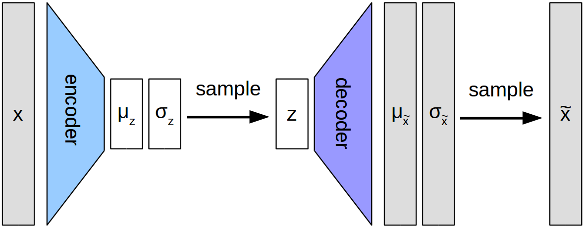
VAE

A simple Variational Auto Encoder using just what we made so far!!

Since we made everything in this from scratch already I will be using Flux directly. (I will attempt to do optimizers in the next post)

Okay so what is that? it is a neural network which is used for things like Image compression, Image generation etc etc. It is cool because it is pretty cheap computationally.

So what do we need to build it?

Architecture

-

• This is the what makes the VAE special. If you notice, the conv sizes first start off huge (Encoder), then reduce to a really small point and then go back up huge again(Decoder).
• So the thing is, the Encoder is responsible for taking the input data and encoding it so to speak into what is called the latent space representation. In human terms it means that it tries to find a very high dimensional representation of the images. Aka it tries to "learn" what the image is so it can recreate it.
• The middle bit which has the smallest sizes is called the bottle neck (because it looks like one lol) and this is what helps in image compression. Since the Convolution and max pool layers fundamentally try to represent images in a very compressed manner, this is the effect. Now the fun part is that we can take the representation space (which the encoder pops things in) and sample from it to get representations of the initial data. These we pop into the decoder.
• The last bit of the architecture is the Decoder which is responsible for giving us back our images (albeit similar and not the same ones). What this does is takes the input as the probability distribution of the data (which is a single pixel in the Bernoulli distribution) and outputs a parameter for every pixel in the image. (aka what it thinks should be the image).

Loss function

• This is a cool looking equation haha. $$ l_i(\Theta,\Phi) = -\mathbb{E}{q\Theta(z|x_i)}[log(p\Theta(x_i|z)] + \mathbb{KL}(q_\Theta(z|x_i) || p(z)) $$

Let us break it down or I will break down.

• $$ l_i(\Theta,\Phi) $$ => Greek way of writing the loss between two things. (Could be x and y if you are not awake yet).
• $$ -\mathbb{E}{q\Theta(z|x_i)}[log(p\Theta(x_i|z)] $$ => likelihood of something happening -> the log of it -> negative of it -> Expected value of all this drama. This lets the network learn that it needs to remake the data again. Since the outputs are probabilities, it is a nice way of seeing how well we did
• $$ \mathbb{KL}(q_\Theta(z|x_i) || p(z)) $$ This is the KL divergence. It is a nice measure to see how far away we are from what we need. Aka how much data is lost in translation so to speak. This acts as a regularizer and reduces the chances of mode collapse (everything is similar so output random nonsesense).

Issues

• A lot of data is lost in translation because the decoder reconstructs from a reduced version of the image.
• Outputs are really blurry (This was fixed in a recent paper. I made notes for it but I havent pushed it yet)

Code

Libraries + data

We load all required libraries. Batch the data and split it to train and test.

using Flux, Flux.Data.MNIST, Statistics, Flux.Optimise
using Flux: throttle, params
X = (float.(hcat(vec.(MNIST.images())...)) .> 0.5) 
N, M = size(X, 2), 100
data = [X[:,i] for i in Iterators.partition(1:N,M)]

Encoder + Bottleneck

We need to pick something from the sampled space and also run our encoder. - (Dense(784, 500, tanh), Dense(500, 5), Dense(500, 5))

Dz, Dh = 5, 500
A, μ, logσ = Dense(28^2, Dh, tanh) , Dense(Dh, Dz) , Dense(Dh, Dz) 

g(X) = (h = A(X); (μ(h), logσ(h)))

function sample_z(μ, logσ)
    eps = randn(Float32, size(μ)) 
    return μ + exp.(logσ) .* eps
end

Decoder aka Generative

We define the decoder here. - Chain(Dense(5, 500, tanh), Dense(500, 784, σ))

f = Chain(Dense(Dz, Dh, tanh), Dense(Dh, 28^2, σ))
kl_q_p(μ, logσ) = 0.5f0 * sum(exp.(2f0 .* logσ) + μ.^2 .- 1f0 .+ logσ.^2)

function logp_x_z(x, z)
    p = f(z)
    ll = x .* log.(p .+ eps(Float32)) + (1f0 .- x) .* log.(1 .- p .+ eps(Float32))
    return sum(ll)
end

L̄(X) = ((μ̂, logσ̂) = g(X); (logp_x_z(X, sample_z(μ̂, logσ̂)) - kl_q_p(μ̂, logσ̂)) * 1 // M)

Loss function

Let us define the loss function. And also attempt to sample from the model.

loss(X) = -L̄(X) + 0.01f0 * sum(x->sum(x.^2), params(f))

function modelsample()  
  ϕ = zeros(Float32, Dz)
  p = f(sample_z(ϕ, ϕ))
  u = rand(Float32, size(p))
  return (u .< p) 
end

Loop de loop

Now for the actual training. I will be using ADAM (yes cheating I know but I am trying really hard to get it done from scratch ): ). Also no GPU.

evalcb = throttle(() -> @show(-L̄(X[:, rand(1:N, M)])), 10)
opt = ADAM()

ps = params(A, μ, logσ, f)

for i = 1:10
  @info "Epoch $i"
  Flux.train!(loss, ps, zip(data), opt, cb=evalcb)
end

Output

Finally let us visualize the outputs. Note that it was only for 10 epochs so it is kinda dumb but well.

using Images

img(x) = Gray.(reshape(x, 28, 28))
sample = hcat(img.([modelsample() for i = 1:10])...)
save("sample.png", sample)

-

Finis